Resolve

The SDSS imaging runs in general overlap each other, yielding multiple detections of the same sources. The “window” and “resolve” algorithms handle these overlaps, to determine the window function of the survey and the unique set of detections to use for a homogeneous sample. The “window” algorithm determines which imaging run should be used for primary detections in each area of sky. Next, the “resolve” algorithm determines which set of detections is “primary,” and finds “secondary” detections of the same sources. There are some sources which are detected but in fields which are not primary; these detections are called “best.”

The BOSS survey targets primary objects for its galaxy and QSO survey. We expect that most users will also want to select the primary sample, unless they are specifically trying to coadd catalog data or looking for time variability.

As usual, there are some minor differences in nomenclature between CAS and the SAS flat files. In particular, in the flatfiles we define resolve_status, image_status, psp_status and thing_id, and in CAS these are resolveStatus, imageStatus, pspStatus and thingID.

The resolve algorithm described here was used for DR8 and later. The same set of resolve results was used in DR8 through DR12. For DR13 and beyond, a new resolve was run accounting for the small changes in astrometry in DR9 and making new decisions about which fields were primary based on the updated calibration in DR13. For the EDR through DR7 a different version of resolve was used that was more specifically tailored to the needs of the Legacy imaging survey.

Starting with DR13, flux calibration is now tied to Pan-STARRS 1 (PS1), resulting in some changes to which detections of sources are considered “primary” for those sources detected more than once. The resolve algorithm itself was not changed. See the imaging caveats page for more details and references.

Using resolve information

Introduction

The results of resolve allow one to perform several tasks. We will describe here: how to define a set of unique objects (that is, with duplicate detections removed); how to find multiple detections of a single object; and, how to describe the geometry of the survey.

Selecting unique objects (removing duplicates)

Users of CAS can select unique objects by using the photoPrimary table, which applies the selection for primary objects across the survey described in this section. Users of the flat files will need to apply these criteria themselves.

The information about how resolve each object is stored in a bitmask called resolve_status (in the flat files) or resolveStatus (in the CAS tables). Notably, SURVEY_PRIMARY is bit 8 (or 2⁸ = 256).

Selecting unique objects from the data is as simple as checking a single bit in this resolve status bitmask The selection can be applied as:

 (resolve_status & SURVEY_PRIMARY) != 0

Equivalently one can check a variable called “mode”, which is set to 1 for primary objects.

In the flat files (either the data sweeps or in the photoObj files) the selection can be applied as:

 (resolve_status & SURVEY_PRIMARY) != 0

If you are interested in just a particular run, you can also ask whether a set of objects are unique within a run (even if they have detections in overlapping runs). The RUN_PRIMARY bit selects such objects, which eliminates duplicates detected in the overlaps between frames in the same camcol (see below):

 (resolve_status & RUN_PRIMARY) != 0

The resolve flags are only set for that unique set of objects that are not further deblended into other objects. In the terminology of SDSS, these are CHILD objects. The CHILD objects can be identified on the basis of the objc_flags bitmask as follows:

 ((objc_flags & BLENDED) == 0  || (objc_flags & NODEBLEND) != 0) && (objc_flags & BRIGHT) == 0

Multiple detections of single objects

The resolve results also allow quick retrieval of multiple detections of single objects. However, the logic is somewhat more involved. For the purposes of this section, we will distinguish between a “source” and a “detection.” A source is a physical source of light in the sky, that might have been detected in more than one field (if more than one field covered that area of sky). A detection is a particular detection of each source. Each entry in the photometric catalog is a detection, and there can be multiple detections for each source, since fields overlap.

First, for each detection, in addition to the resolve status bits, there are indicators of how many fields that object could have been detected in (NOBSERVE) and of how many fields that object actually was detected in (NDETECT) The photoObj flat files and the photoObjAll table in CAS both have this information.

Second, for each unique source, we assign a unique identification number called thing_id. All detections associated with that source have that same value of thing_id associated with them.

To actually find the multiple detections of a single source, the method differs between the FITS flat files and the CAS.

In the flat-file distribution, we provide two files. One contains all of the detections (thingList) and one which contains all of the unique sources (thingIndex). In fact, thing_id simply is equal to the zero-indexed row of thingIndex that contains the information about that source. In thingIndex is listed (as ISTART) the first occurrence of a detection in thingList; all of the detections of individual sources are grouped together, so along with NDETECT this yields enough information to find all of the detections.

Thus, say you have a primary detection of some source, and want to find the list of all detections of that source. Then you look in thingIndex[thing_id] for ISTART and NDETECT. The information about all of the other detections can then be found in the elements thingList[ISTART...ISTART+NDETECT]. In those elements are listed the RUN, CAMCOL, FIELD, and ID of all of the detections.

For CAS, we provide the same information in two tables: detectionIndex (which corresponds to the thingList file) and thingIndex (which corresponds to the (thingIndex file). thingIndex provides the full list of unique sources. detectionIndex provides pairs of objId and thingID. Thus, with known thingIds, one can join to all the photometric information in photoObj for each detection using the detectionIndex table.

Geometry of survey

As we explain below, in each direction on the sky covered by SDSS data, we have chosen one field covering it as primary. Over about two-thirds of the are there is single-field coverage, but about one-third of the time there are two or more fields and a choice must be made. Here we describe the tools to use this information, using the flat-files, using the SAS front-end, and using the CAS database.

The essential information expressing the primary field coverage is contained in the window_unified.fits and window_flist.fits files. window_unified.fits is a FITS-format file with a Mangle-style geometry in it. idlutils users can read it in with read_fits_polygons. It contains a set of polygons; the parameter “IFIELD” is an index into the window_flist.fits file that indicates which field is primary in that polygon.

The SAS front-end also provides an interface to the same information, allowing the user to check the primary field covering a particular RA and Dec or a list.

In CAS, the window function information is encoded in the sdssPolygons table. The best way to use that table is with the special geometry functions within CAS. The sample queries give an example of testing the SDSS footprint.

Resolve algorithm

Introduction and nomenclature

The catalogs generated by the SDSS imaging camera and the photometric pipeline often contains areas of sky which have been covered multiple times. Thus, to evaluate the sky coverage of the survey and to define a unique set of detected objects requires understanding these overlaps. We refer to our description of the sky coverage as the “window” of the SDSS survey, and we refer to the process of identifying duplicate observations as “resolving” the catalog.

We will refer to the unique coverage of the survey as the “primary” area. The primary area is built up as a union of the individual SDSS fields. At each position in that area there is a single field deemed “primary.” For each field, some parts of it might be primary and others not. We will show examples below.

We will refer to individual detections in a field as a “detection” or a “catalog entry.” Only detections that are in the primary area of a field are classified as “primary”. Detections in a non-primary part of a field are usually called “secondary.” Some unique detections exist but in areas of fields where that field is not primary; that is, cases where a secondary observation of an area contains a detection whereas the primary field covering that area does not. Such cases are called “best”.

Geometry of a run

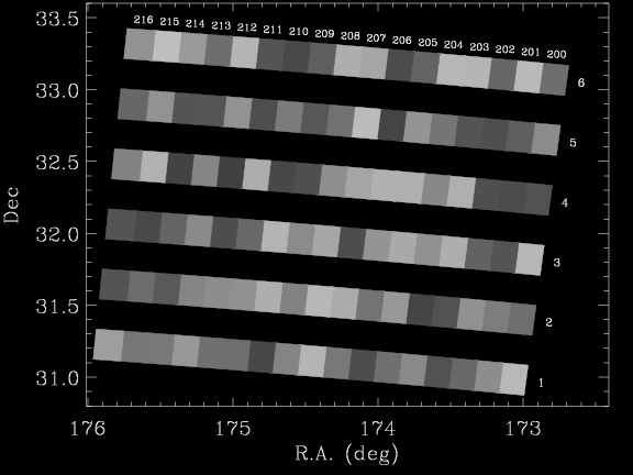
The SDSS imaging data set is built up from a series of drift scan runs, ranging from an hour to over eight hours in length. The scan rate across the sky is similar to the sidereal rate on the equator. During each run, images are taken in six long, narrow camcols on the sky, about 13.5 arcmin in width. The camcols are separated from each other by slightly less than their 13.5 arcmin width. Each camcol is divided into individual fields that 9.8 arcmin long. Each overlaps by about 50 arcsec with the next field and the previous field. In pixel units, each field is 2048 columns by 1489 rows, with 128 rows overlap with the previous and next field (0.396 arcsec per pixel).

For each field, there is an image in each of the five bands (u, g, r, i, and z) taken within a few minutes of each other. The photometric reduction software processes each field mostly independently.

The figure above shows an image of the coverage of part of an SDSS run. Each field is denoted by its run, camcol, and field numbers, which fully identify it. Note the gaps between the camcols. Generally speaking, the gaps are filled with imaging from runs that run nearly parallel.

As a first step in defining the geometry of the full survey, we define the official area covered by each field. This is the full area of the corrected frame (2048x1489) with 64 pixels trimmed off of each edge. The trimming along the drift scan direction prevents adjacent fields from overlapping. The trimming perpendicular to the drift scan direction prevents objects that are too close to the frame edge from entering the primary catalog; these objects near the edge are often incorrectly analyzed by the photo software, and thus best left out of the primary sample.

Distribution of fields on the sky

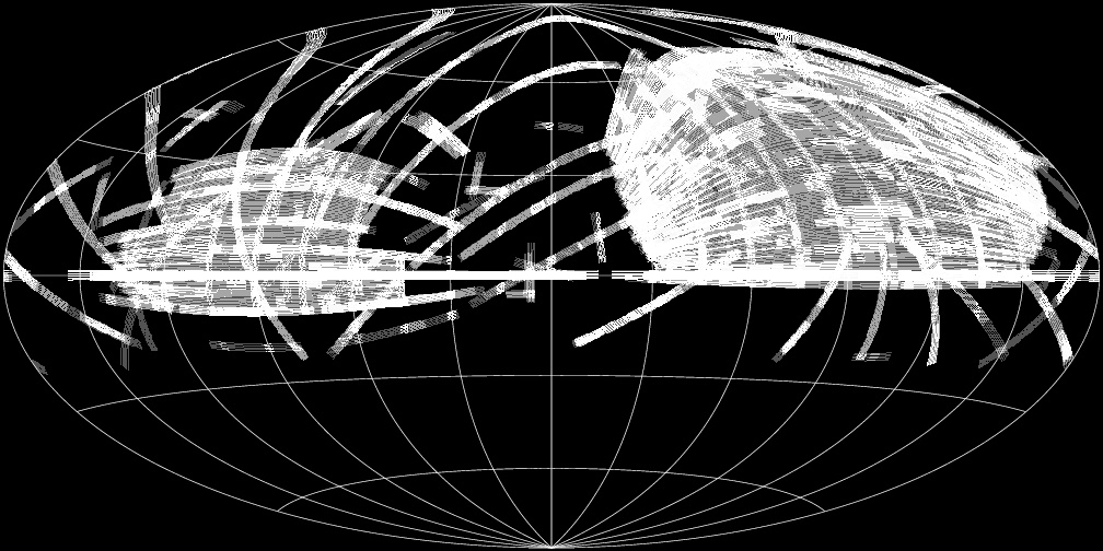
Next we show the distribution of all the individual fields on the sky for the full survey. The shading as a function of position indicates the number of fields covering each position.

The survey has defined a set of standard “stripes” which most (though not all) of the runs can be associated with. In this case, the full stripe is imaged with runs in two “strips”, one identified as the “north” strip and one as the “south” strip. Each stripe has an integer number associated with it, so runs are identified as being part of strip “11N” or “82S” or the like.

Most of the stripes lie on great circles with a common pole at a right ascension of 95 deg and a declination of 0 deg, which lies outside the main survey near the Galactic Plane. For this reason, the stripes actually overlap each other considerably near the survey edges.

Obviously, many objects that lie in regions covered more than once will be detected multiple times. The purpose of resolve is to identify such cases and remove duplicates.

Scoring the fields

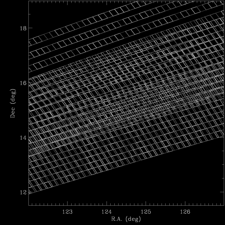
In each region shown in the above figure, there are one or more fields covering the area. We strive to pick the best possible field to represent each area. As the first step to doing so, we have to rank the fields according to some metric, which we call the field “score.”

For normal SDSS runs, the formula for the score is:

 sensitivity = (0.7 / (PSF_FWHM[2] * sqrt(SKYFLUX[2]))) < 0.4 score = QEXIST * (0.1 + 0.5 * QPHOT + sensitivity)

where sensitivity is bounded between [0,0.4], and measures the point-source sensitivity according to the FWHM and the sky level in the r-band.

A field is considered to exist (QEXIST) if photoStatus is 0 (that is, the photometric reductions were completed) and image_status doesn’t have any of the following bits set in any band: BAD_ROTATOR, BAD_ASTROM, BAD_FOCUS, or SHUTTERS.

A field is considered photometric (QPHOT) if it is darker than 12 deg twi in the r-band, if the postage stamp pipeline did not return errors in any band (that is, if psp_status is <= 2 (in the lower 5 bits), which rejects PSP_FIELD_NOPSF, PSP_FIELD_ABORTED, PSP_FIELD_MISSING, PSP_FIELD_OE_TRANSIENT), and if image_status doesn’t have any of the bits set in any band: CLOUDY, UNKNOWN, FF_PETALS, DEAD_CCD, or NOISY_CCD.

Therefore, the possible values of the score are:

 [0]         -- No data or un-reducable data (0.1 ,0.5 ] -- Unphotometric data (0.6 ,1   ] -- Photometric data

The range between 0 and 0.1 is reserved for fast “binned” Apache Wheel drift scans used in the calibration of the survey.

Geometry of the primary survey

As noted above, the primary survey area is defined as the union of all of the fields. Determining this area requires two steps: first, determining for each position on the sky which fields cover it; second, at each position determine which field should be considered primary.

To determine which fields cover which positions, we treat each field as a four-sided spherical polygon on the sky defined by its trimmed area as described above (which is 1920x1361 pixels in size). For an example case, the figure shows the boundaries of all the fields. Notice that there is a unique set of disjoint polygons on the sky defined by all the field boundaries. In fact, one can calculate exactly what all those polygons are using the package mangle. We refer to them here as “balkans.” Each field is broken into several balkans, and each balkan is fully covered by a single combination of one or more fields.

Then, for each balkan we determine which field that covers it is primary. We start with the highest ranked field. It becomes primary for any balkan covered by it. Then we step to its adjacent fields in the same run and camcol. As long as their score is within 0.05 of the initial field we assign them primary to the balkans they cover as well. We continue along the camcol in both direction until we reach a substantially worse field than the first. Once that is done, we then step to the next highest ranked field that has not already been assigned. We execute the same steps for that field. Finally, we iterate this procedure until we have assigned all of the fields. During this procedure, if a balkan has already been assigned a primary field, that assignment is not change.

The result is that for any area, the highest score fields that cover it will most likely be primary. The reason we step through the surrounding fields is to avoid changing between two comparably good runs on the same strip; for homogeneity, it is better just to pick one and go with it if the different in quality is not too large.

Resolving catalog detections

Once the window function is defined, we can resolve multiple detections of individual objects. This proceeds in four steps:

1. defining the set of “run primary” detections, unique in each run and selected as RUN_PRIMARY as described above;
2. defining the set of “survey primary” detections, unique across the survey as a whole and detected in the primary area of field and selected as SURVEY_PRIMARY as described above;
3. defining the set of “best” detections, unique in the survey as a whole but with no detection in the primary field covering its position, and selected as SURVEY_BEST using resolve_status; and
4. defining the set of secondary detections, duplicate detections of survey primary detections, and selected as SURVEY_SECONDARY using resolve_status.

The first step is the “run resolve” step, where duplicates between adjacent fields in a run are resolved. In this step, we select objects which are in the 2048x1361 central area of the corrected frame for the field, as described above. However, along the edges in the drift scan direction, we take care to account for small astrometric differences that might cause lost or duplicate objects. To do so, if any two detections in adjacent fields are within 2 arcsec of each other and straddle an edge, one and only one of them is chosen as primary for the run. For objects that pass these selection cuts, the RUN_PRIMARY bit of resolve_status is set.

Note that RUN_PRIMARY objects within 64 pixels of the boundary perpendicular to the scan edge (columns 0 to 63 and 1984 to 2047) are marked RUN_EDGE. RUN_EDGE objects in almost all cases do not become SURVEY_PRIMARY.

In addition, we do not allow any RUN_PRIMARY objects which are parents, are classified as BRIGHT detections, or have been classified as “SKY” or “CR” in the “type” indicator. This exclusion also means that such objects can never be primary for the full survey either.

The second step is to define the “survey primary” detections, which is a list of unique detections among all the runs. In each area of sky, detections can only be primary if they are from the primary field in that direction as defined by the window function above. To find this set of objects, we loop over all the balkans defining the survey geometry. From the primary field covering each balkan, we select RUN_PRIMARY detections that are within the balkan, or within 1 arcsec of the edge. In this step we ignore RUN_EDGE objects (mostly! see next paragraph). We match each selected detection to the current list of primary detections. If it matches a previous primary detection, as it might if it is near the edge of the balkan, then we do not include it (this step accounts for small astrometric jitter between adjacent balkans). Otherwise it is called SURVEY_PRIMARY in resolve_status.

As this procedure is performed, we are also careful to check detections that are close to, but outside, the “official” boundaries perpendicular to the scan direction. That is, we check those marked RUN_EDGE but within 1 arcsec of the border. Sometimes it happens that there are multiple detections of the same source from different runs, but both detections are in this tiny strip. Rather than lose such objects, we flag the one in the higher quality field as SURVEY_PRIMARY.

The third step is to define the “survey best” detections, which is a list of unique detections, but in cases where there is no detection of the source in the primary field covering it. Such cases can occur for transient or low signal-to-noise sources, where it is detected in some fields observing it but not in others. To find such objects, we loop over all the fields, and match all of the RUN_PRIMARY objects to the full list of SURVEY_PRIMARY objects. Objects that are unmatched are good detections in this field, but have no corresponding primary objects, and are labeled as SURVEY_BEST in resolve_status.

Finally, the last step is to define the “survey secondary” detections, which are the duplicate detections of primary or best objects. To find such objects, we loop over all fields and select objects which are RUN_PRIMARY but neither SURVEY_PRIMARY nor SURVEY_BEST. We match these objects against the SURVEY_PRIMARY and SURVEY_BEST lists (excluding objects in this field). If it is matched, and the balkan containing the primary/best observation contains the current field we are considering, then this detection is labeled SURVEY_SECONDARY.

As these procedures are run, we create the thingList and thingIndex files. thingList has all of the detections in it and labels its status (e.g. SURVEY_PRIMARY, SURVEY_BEST or SURVEY_SECONDARY) as well as listing the thing_id of its primary if appropriate. thingIndex is a list of all unique detections, listing the SURVEY_PRIMARY or SURVEY_BEST detection as appropriate. Above we describe how to use these files to find primaries and to find multiple detections of each object.

At the end of the process, most RUN_PRIMARY detections have one of SURVEY_PRIMARY, SURVEY_BEST or SURVEY_SECONDARY set. The only exceptions are those RUN_PRIMARY objects which also have RUN_EDGE set; while such objects can have a survey status, they do not have to.

Toy example

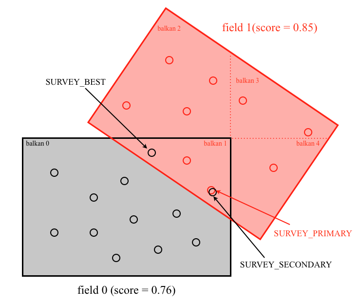
The basics of the algorithm can be illustrated with a toy example, shown above. There are two fields in this toy survey, which overlap. The geometry is broken up into five balkans (not three, since each balkan must be convex). In this case, in four of the balkans, there is only a single field. In the other one, balkan 1, there are two fields covering the area. The better field is chosen as primary.

In this case, the window_unified.fits file would have 5 entries. For one of them, balkan 0, IFIELD would be set to 0, and for balkans 1 through 4, IFIELD would be set to 1.

Shown in the figure are the RUN_PRIMARY objects detected in each field. Those which are in the area of their field which is primary will become SURVEY_PRIMARY (that is, all of the field 1 objects, and the field 0 objects which are in balkan 0).

In this case, there are two objects detected in field 0 that are in the overlap between the two fields, where field 0 is not primary. One object matches a field 1 SURVEY_PRIMARY object, and thus is called SURVEY_SECONDARY. It will be given the same THING_ID as the corresponding field 1 object. The other object does not match any field 1 SURVEY_PRIMARY object; this is a case that will be flagged SURVEY_BEST. Finally, note that there is a field 1 object with no matching field 0 object.

Caveats

A very rare case occurs for objects just outside of the first or last field of a run in the scan direction, where the object must be included in analogy to the RUN_EDGE case described above. In exactly one case such an object has not been designated RUN_PRIMARY but is designated SURVEY_PRIMARY, which is the only example of that in the survey.